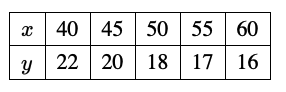
Abi and Bhani find the fuel consumption for a car driven at different constant speeds. The table shows the fuel consumption, $y$ kilometres per litre, for different constant speeds, $x$ kilometres per hour.
(i) Abi decides to model the data using the line $y=35-\frac{1}{3} x$.
(a) On the grid opposite
- draw a scatter diagram of the data,
- draw the line $y=35-\frac{1}{3} x$.
[2]
(b) For a line of best fit $y=\mathrm{f}(x)$, the residual for a point $(a, b)$ plotted on the scatter diagram is the vertical distance between $(a, \mathrm{f}(a))$ and $(a, b)$. Mark the residual for each point on your diagram.
[1]
(c) Calculate the sum of the squares of the residuals for Abi’s line.
[1]
(d) Explain why, in general, the sum of the squares of the residuals rather than the sum of the residuals is used.
[1]
Bhani models the same data using a straight line passing through the points $(40,22)$ and $(55,17)$. The sum of the squares of the residuals for Bhani’s line is 1 .
(ii) State, with a reason, which of the two models, Abi’s or Bhani’s, gives a better fit.
[1]
(iii) State the coordinates of the point that the least squares regression line must pass through.
[1]
(iv) Use your calculator to find the equation of the least squares regression line of $y$ on $x$. State the value of the product moment correlation coefficient.
[3]
(v) Use the equation of the regression line to estimate the fuel consumption when the speed is 30 kilometres per hour. Explain whether you would expect this value to be reliable.
[2]
(vi) Cerie performs a similar experiment on a different car. She finds that the sum of the squares of the residuals for her line is 0 . What can you deduce about the data points in Cerie’s experiment?
[1]